Example 1:Hinge and Square Loss

This example try to show how to use our PLQ Composite Decomposition tool to decompose a given loss function and use ReHLine to do classification.

Given a loss function \(L(z)=\max(\max(1-z,0)),\frac{1}{2} (1-z)^2 )\)

import numpy as np

z = np.linspace(-2, 2, 100)
L1 = np.maximum(1 - z, 0)
L2 = 0.5 * (1 - z) ** 2

import matplotlib.pyplot as plt

plt.figure(figsize=(4, 3))
plt.plot(z, L1, marker='o', label='Hinge Loss')
plt.plot(z, L2, marker='s', label='Square Loss')
plt.plot(z, np.maximum(L1, L2), marker='^', label='PLQ Loss')
plt.legend()
plt.xlabel('z')
plt.ylabel('L(z)')
plt.title('Hinge Loss and Square Loss')
plt.show()

1.Data Generation

from plqcom import PLQLoss, plq_to_rehloss, affine_transformation
from rehline import ReHLine
from rehline._base import _relu, _rehu

Generate a random classification dataset, where \(\mathbf{X} \in \mathbb{R}^{1000 \times 3}\) and \(\mathbf{y} \in \mathbb\{ -1, 1\}^{1000}\)

# Generate a random classification dataset
n, d, C = 1000, 3, 0.5
np.random.seed(1024)
X = np.random.randn(n, d)
beta = np.random.randn(d)
y = np.sign(X.dot(beta) + np.random.randn(n))

First 10 samples of the dataset

X[:10], y[:10]

(array([[ 2.12444863,  0.25264613,  1.45417876],
        [ 0.56923979,  0.45822365, -0.80933344],
        [ 0.86407349,  0.20170137, -1.87529904],
        [-0.56850693, -0.06510141,  0.80681666],
        [-0.5778176 ,  0.57306064, -0.33667496],
        [ 0.29700734, -0.37480416,  0.15510474],
        [ 0.70485719,  0.8452178 , -0.65818079],
        [ 0.56810558,  0.51538125, -0.61564998],
        [ 0.92611427, -1.28591285,  1.43014026],
        [-0.4254975 , -0.40257712,  0.60410409]]),
 array([ 1., -1., -1., -1., -1.,  1., -1., -1.,  1.,  1.]))

X[:10].dot(beta)

array([ 4.63095617, -1.53086335, -3.77183917,  1.49927261, -1.1677152 ,
        0.56448038, -1.12647624, -1.09186115,  3.93541798,  1.1463427 ])

2. Create and Decompose the PLQ Loss

Create the PLQ Loss object with the given quad_coef only (max form).

plqloss_1 = PLQLoss(
    quad_coef={'a': np.array([0., 0., 0.5]), 'b': np.array([0., -1., -1.]), 'c': np.array([0., 1., 0.5])},
    form='max')

We can also create the PLQ Loss object with the given quad_coef and cutpoints.(plq form)

plqloss_2 = PLQLoss(
    quad_coef={'a': np.array([0.5, 0., 0.5]), 'b': np.array([-1., -1., -1.]), 'c': np.array([0.5, 1., 0.5])},
    cutpoints=np.array([-1., 1.]),
    form='plq')

Convert the PLQ Loss to ReHLoss by calling its method plq_to_rehloss)

rehloss_1 = plq_to_rehloss(plqloss_1)
rehloss_2 = plq_to_rehloss(plqloss_2)

rehloss_1.relu_coef, rehloss_1.relu_intercept, rehloss_1.rehu_cut, rehloss_1.rehu_coef, rehloss_1.rehu_intercept
rehloss_2.relu_coef, rehloss_2.relu_intercept, rehloss_2.rehu_cut, rehloss_2.rehu_coef, rehloss_2.rehu_intercept

(array([[-1.],
        [-1.]]),
 array([[ 1.],
        [-1.]]),
 array([[inf],
        [inf]]),
 array([[-1.],
        [ 1.]]),
 array([[-1.],
        [-1.]]))

rehloss_1.rehu_coef == rehloss_2.rehu_coef

array([[ True],
       [ True]])

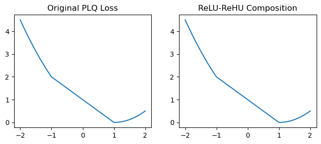
plt.figure(figsize=(8, 3))
plt.subplot(1, 2, 1)
Z = np.linspace(-2, 2, 1000)
L = plqloss_1(Z)
plt.plot(Z, L)
plt.title('Original PLQ Loss')

plt.subplot(1, 2, 2)
relu_coef, relu_intercept = rehloss_1.relu_coef, rehloss_1.relu_intercept
rehu_cut, rehu_coef, rehu_intercept = rehloss_1.rehu_cut, rehloss_1.rehu_coef, rehloss_1.rehu_intercept
Reh = np.sum(_rehu(rehu_coef * Z + rehu_intercept, rehu_cut), axis=0) + np.sum(_relu(relu_coef * Z + relu_intercept),
                                                                              axis=0)
plt.plot(Z, Reh)
plt.title('ReLU-ReHU Composition')
plt.show()

3.Broadcast to all samples

For this classication problem, \(L(z)= \max(\max(1-z,0)),\frac{1}{2} (1-z)^2 )\) \(L_i(z_i)=\frac{1}{2} \max(\max(1-y_i z_i,0)),\frac{1}{2} (1-y_i z_i)^2 )\) Compare \(L_i(z_i)\) with \(L(z)\), we can find that \(L_i(z_i)=\frac{1}{2}L(y_i z_i)\) which is a affine transformation of \(L(z)\) with \(p=y_i, q=0,c=\frac{1}{2}\).

rehloss = affine_transformation(rehloss_1, n=X.shape[0], c=C, p=y, q=0)

print(rehloss.relu_coef, rehloss.relu_intercept, rehloss.rehu_cut, rehloss.rehu_coef, rehloss.rehu_intercept)

[[-0.5  0.5  0.5 ...  0.5  0.5 -0.5]
 [-0.5  0.5  0.5 ...  0.5  0.5 -0.5]] [[ 0.5  0.5  0.5 ...  0.5  0.5  0.5]
 [-0.5 -0.5 -0.5 ... -0.5 -0.5 -0.5]] [[inf inf inf ... inf inf inf]
 [inf inf inf ... inf inf inf]] [[-0.70710678  0.70710678  0.70710678 ...  0.70710678  0.70710678
  -0.70710678]
 [ 0.70710678 -0.70710678 -0.70710678 ... -0.70710678 -0.70710678
   0.70710678]] [[-0.70710678 -0.70710678 -0.70710678 ... -0.70710678 -0.70710678
  -0.70710678]
 [-0.70710678 -0.70710678 -0.70710678 ... -0.70710678 -0.70710678
  -0.70710678]]

4. Use ReHLine to solve the problem

clf = ReHLine()
clf.U, clf.V, clf.Tau, clf.S, clf.T, clf.C = rehloss.relu_coef, rehloss.relu_intercept, rehloss.rehu_cut, rehloss.rehu_coef, rehloss.rehu_intercept, C
clf.fit(X=X)
print('sol privided by rehline: %s' % clf.coef_)
print('decision_function: %s' % clf.decision_function([[.1, .2, .3]]))
print('precision: %s' % (np.sum(np.sign(X.dot(clf.coef_)) == y) / n))

sol privided by rehline: [ 0.20339926 -0.00843538  0.69527244]
decision_function: [0.22723458]
precision: 0.868